UTS Data Mining#

Klasifikasi Data Pada Dataset Breats Cancer#

Lakukan analisa terhadap data pada https://archive.ics.uci.edu/ml/datasets/Breast+Cancer+Coimbra dengan menggunakan klasifikasi

Metode KNN
Metode pohon keputusan (Desision tree)

Data#

import numpy as np
import matplotlib.pyplot as plt
import seaborn as sns
import numba
import cv2 as cv
import pandas as pd
from sklearn.decomposition import PCA
from sklearn.neighbors import KNeighborsClassifier
from sklearn.metrics import confusion_matrix
from sklearn.model_selection import train_test_split
from sklearn.metrics import classification_report
from sklearn.tree import DecisionTreeClassifier
from sklearn.metrics import accuracy_score
from sklearn import tree
from matplotlib import pyplot as plt 

data = pd.read_csv("https://raw.githubusercontent.com/LALA09-erha/Python-StrukturData/master/dataR2.csv")
data_1 = pd.read_csv("https://raw.githubusercontent.com/LALA09-erha/Python-StrukturData/master/dataR2.csv")
data

	Age	BMI	Glucose	Insulin	HOMA	Leptin	Adiponectin	Resistin	MCP.1	Classification
0	48	23.500000	70	2.707	0.467409	8.8071	9.702400	7.99585	417.114	1
1	83	20.690495	92	3.115	0.706897	8.8438	5.429285	4.06405	468.786	1
2	82	23.124670	91	4.498	1.009651	17.9393	22.432040	9.27715	554.697	1
3	68	21.367521	77	3.226	0.612725	9.8827	7.169560	12.76600	928.220	1
4	86	21.111111	92	3.549	0.805386	6.6994	4.819240	10.57635	773.920	1
...	...	...	...	...	...	...	...	...	...	...
111	45	26.850000	92	3.330	0.755688	54.6800	12.100000	10.96000	268.230	2
112	62	26.840000	100	4.530	1.117400	12.4500	21.420000	7.32000	330.160	2
113	65	32.050000	97	5.730	1.370998	61.4800	22.540000	10.33000	314.050	2
114	72	25.590000	82	2.820	0.570392	24.9600	33.750000	3.27000	392.460	2
115	86	27.180000	138	19.910	6.777364	90.2800	14.110000	4.35000	90.090	2

116 rows × 10 columns

Ubah Label 1=Healthy controls dan 2=Patients#

data_1['Classification'] = data_1['Classification'].apply({1:'Healthy controls', 2:'Patients'}.get)
data_1

	Age	BMI	Glucose	Insulin	HOMA	Leptin	Adiponectin	Resistin	MCP.1	Classification
0	48	23.500000	70	2.707	0.467409	8.8071	9.702400	7.99585	417.114	Healthy controls
1	83	20.690495	92	3.115	0.706897	8.8438	5.429285	4.06405	468.786	Healthy controls
2	82	23.124670	91	4.498	1.009651	17.9393	22.432040	9.27715	554.697	Healthy controls
3	68	21.367521	77	3.226	0.612725	9.8827	7.169560	12.76600	928.220	Healthy controls
4	86	21.111111	92	3.549	0.805386	6.6994	4.819240	10.57635	773.920	Healthy controls
...	...	...	...	...	...	...	...	...	...	...
111	45	26.850000	92	3.330	0.755688	54.6800	12.100000	10.96000	268.230	Patients
112	62	26.840000	100	4.530	1.117400	12.4500	21.420000	7.32000	330.160	Patients
113	65	32.050000	97	5.730	1.370998	61.4800	22.540000	10.33000	314.050	Patients
114	72	25.590000	82	2.820	0.570392	24.9600	33.750000	3.27000	392.460	Patients
115	86	27.180000	138	19.910	6.777364	90.2800	14.110000	4.35000	90.090	Patients

116 rows × 10 columns

type(data)

pandas.core.frame.DataFrame

Metode KNN Clafification#

split data

data.shape

(116, 10)

memisahkan data dengan kelas ke dalam dua variabel, X dan y

X = data.drop(columns=["Classification"])
X.head()

	Age	BMI	Glucose	Insulin	HOMA	Leptin	Adiponectin	Resistin	MCP.1
0	48	23.500000	70	2.707	0.467409	8.8071	9.702400	7.99585	417.114
1	83	20.690495	92	3.115	0.706897	8.8438	5.429285	4.06405	468.786
2	82	23.124670	91	4.498	1.009651	17.9393	22.432040	9.27715	554.697
3	68	21.367521	77	3.226	0.612725	9.8827	7.169560	12.76600	928.220
4	86	21.111111	92	3.549	0.805386	6.6994	4.819240	10.57635	773.920

#separate target values
y = data["Classification"].values
#view target values
y[0:150]

array([1, 1, 1, 1, 1, 1, 1, 1, 1, 1, 1, 1, 1, 1, 1, 1, 1, 1, 1, 1, 1, 1,
       1, 1, 1, 1, 1, 1, 1, 1, 1, 1, 1, 1, 1, 1, 1, 1, 1, 1, 1, 1, 1, 1,
       1, 1, 1, 1, 1, 1, 1, 1, 2, 2, 2, 2, 2, 2, 2, 2, 2, 2, 2, 2, 2, 2,
       2, 2, 2, 2, 2, 2, 2, 2, 2, 2, 2, 2, 2, 2, 2, 2, 2, 2, 2, 2, 2, 2,
       2, 2, 2, 2, 2, 2, 2, 2, 2, 2, 2, 2, 2, 2, 2, 2, 2, 2, 2, 2, 2, 2,
       2, 2, 2, 2, 2, 2])

Memisahkan Data Training dan Test#

from sklearn.model_selection import train_test_split
#split dataset into train and test data
X_train, X_test, y_train, y_test = train_test_split(X, y, test_size=0.2, random_state=1, stratify=y)

membuat Model#

Dengan menetapkan N = 3 atau 3 tetangga

from sklearn.neighbors import KNeighborsClassifier
# Create KNN classifier
knn = KNeighborsClassifier(n_neighbors = 3)
# Fit the classifier to the data
knn.fit(X_train,y_train)

KNeighborsClassifier(n_neighbors=3)

Melakukan testing data pada model#

#show first 5 model predictions on the test data
knn.predict(X_test)[1:25]

array([2, 1, 2, 2, 1, 2, 1, 2, 2, 2, 1, 1, 1, 1, 2, 2, 2, 1, 2, 2, 2, 2,
       2])

Menghitung akurasi yang didapat#

#check accuracy of our model on the test data
knn.score(X_test, y_test)

0.3333333333333333

Melakukan K-Fold Cross Validation#

from sklearn.model_selection import cross_val_score
import numpy as np
#create a new KNN model
knn_cv = KNeighborsClassifier(n_neighbors=6)
#train model with cv of 5 
cv_scores = cross_val_score(knn_cv, X, y, cv=5)
#print each cv score (accuracy) and average them
print(cv_scores)
print("cv_scores mean:{}".format(np.mean(cv_scores)))

[0.45833333 0.60869565 0.47826087 0.43478261 0.43478261]
cv_scores mean:0.4829710144927536

Hypertuning model parameters menggunakan GridSearchCV#

from sklearn.model_selection import GridSearchCV
#create new a knn model
knn2 = KNeighborsClassifier()
#create a dictionary of all values we want to test for n_neighbors
param_grid = {'n_neighbors': np.arange(1, 25)}
#use gridsearch to test all values for n_neighbors
knn_gscv = GridSearchCV(knn2, param_grid, cv=5)
#fit model to data
knn_gscv.fit(X, y)

GridSearchCV(cv=5, estimator=KNeighborsClassifier(),
             param_grid={'n_neighbors': array([ 1,  2,  3,  4,  5,  6,  7,  8,  9, 10, 11, 12, 13, 14, 15, 16, 17,
       18, 19, 20, 21, 22, 23, 24])})

Mengecek `n` yang terbaik#

#check top performing n_neighbors value
knn_gscv.best_params_

{'n_neighbors': 23}

Mengecek Hasil dari `n` yang terbaik#

#check mean score for the top performing value of n_neighbors
knn_gscv.best_score_

0.5688405797101449

Kesimpulan#

Dari Hasil diatas bahwa n yang terbaik yaitu 23 dengan hasil 0.5688405797101449

Metode Decision Tree#

data

	Age	BMI	Glucose	Insulin	HOMA	Leptin	Adiponectin	Resistin	MCP.1	Classification
0	48	23.500000	70	2.707	0.467409	8.8071	9.702400	7.99585	417.114	1
1	83	20.690495	92	3.115	0.706897	8.8438	5.429285	4.06405	468.786	1
2	82	23.124670	91	4.498	1.009651	17.9393	22.432040	9.27715	554.697	1
3	68	21.367521	77	3.226	0.612725	9.8827	7.169560	12.76600	928.220	1
4	86	21.111111	92	3.549	0.805386	6.6994	4.819240	10.57635	773.920	1
...	...	...	...	...	...	...	...	...	...	...
111	45	26.850000	92	3.330	0.755688	54.6800	12.100000	10.96000	268.230	2
112	62	26.840000	100	4.530	1.117400	12.4500	21.420000	7.32000	330.160	2
113	65	32.050000	97	5.730	1.370998	61.4800	22.540000	10.33000	314.050	2
114	72	25.590000	82	2.820	0.570392	24.9600	33.750000	3.27000	392.460	2
115	86	27.180000	138	19.910	6.777364	90.2800	14.110000	4.35000	90.090	2

116 rows × 10 columns

Membuat Model Clasifier Decision Tree#

y = data["Classification"]
X = data.drop(columns=["Classification"])
clf = tree.DecisionTreeClassifier(criterion="gini")
clf = clf.fit(X, y)

data.value_counts

<bound method DataFrame.value_counts of      Age        BMI  Glucose  Insulin      HOMA   Leptin  Adiponectin  \
   48  23.500000       70    2.707  0.467409   8.8071     9.702400   
   83  20.690495       92    3.115  0.706897   8.8438     5.429285   
   82  23.124670       91    4.498  1.009651  17.9393    22.432040   
   68  21.367521       77    3.226  0.612725   9.8827     7.169560   
   86  21.111111       92    3.549  0.805386   6.6994     4.819240   
..   ...        ...      ...      ...       ...      ...          ...   
 45  26.850000       92    3.330  0.755688  54.6800    12.100000   
 62  26.840000      100    4.530  1.117400  12.4500    21.420000   
 65  32.050000       97    5.730  1.370998  61.4800    22.540000   
 72  25.590000       82    2.820  0.570392  24.9600    33.750000   
 86  27.180000      138   19.910  6.777364  90.2800    14.110000   

     Resistin    MCP.1  Classification  
   7.99585  417.114               1  
   4.06405  468.786               1  
   9.27715  554.697               1  
  12.76600  928.220               1  
  10.57635  773.920               1  
..        ...      ...             ...  
10.96000  268.230               2  
 7.32000  330.160               2  
10.33000  314.050               2  
 3.27000  392.460               2  
 4.35000   90.090               2  

[116 rows x 10 columns]>

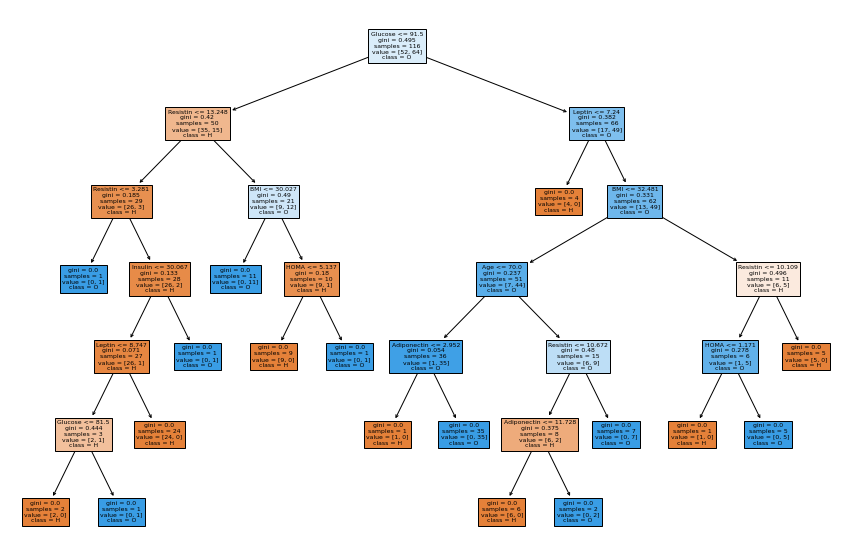
Membuat Grafik Decision Tree dari hasil Klasifikasi#

fig = plt.figure(figsize=(15,10))
_ = tree.plot_tree(clf, feature_names=list(data.columns.values)[:9], class_names=list(data.columns.values)[4] ,filled=True)

Fikri Ainun Najib

UTS Data Mining

Contents

UTS Data Mining#

Klasifikasi Data Pada Dataset Breats Cancer#

Data#

Ubah Label 1=Healthy controls dan 2=Patients#

Metode KNN Clafification#

Memisahkan Data Training dan Test#

membuat Model#

Melakukan testing data pada model#

Menghitung akurasi yang didapat#

Melakukan K-Fold Cross Validation#

Hypertuning model parameters menggunakan GridSearchCV#

Mengecek `n` yang terbaik#

Mengecek Hasil dari `n` yang terbaik#

Kesimpulan#

Metode Decision Tree#

Membuat Model Clasifier Decision Tree#

Membuat Grafik Decision Tree dari hasil Klasifikasi#

Fikri Ainun Najib

UTS Data Mining

Contents

UTS Data Mining#

Klasifikasi Data Pada Dataset Breats Cancer#

Data#

Ubah Label 1=Healthy controls dan 2=Patients#

Metode KNN Clafification#

Memisahkan Data Training dan Test#

membuat Model#

Melakukan testing data pada model#

Menghitung akurasi yang didapat#

Melakukan K-Fold Cross Validation#

Hypertuning model parameters menggunakan GridSearchCV#

Mengecek n yang terbaik#

Mengecek Hasil dari n yang terbaik#

Kesimpulan#

Metode Decision Tree#

Membuat Model Clasifier Decision Tree#

Membuat Grafik Decision Tree dari hasil Klasifikasi#

Mengecek `n` yang terbaik#

Mengecek Hasil dari `n` yang terbaik#